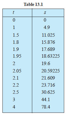
Physical experiments have confirmed that the body dropped from a tall cliff covers a distance of `4.9t^2` metres in t seconds, i.e., distance `s` in metres covered by the body as a function of time `t` in seconds is given by `s = 4.9t^2.`

The adjoining Table 13.1 gives the distance travelled in metres at various intervals of time in seconds of a body dropped from a tall cliff.



The objective is to find the veloctiy of the body at time `t = 2` seconds from this data. One way to approach this problem is to find the average velocity for various intervals of time ending at `t = 2` seconds and hope that these throw some light on the velocity at `t = 2` seconds.

Average velocity between `t = t_1` and `t = t_2` equals distance travelled between `t = t_1` and `t = t_2` seconds divided by `(t_2 – t_1).` Hence the average velocity in the first two seconds

`= ( "Distance travelled between "t = t_2" and "t = t_1 ) /["Time interval " (t_2 – t_1)]`

`= [(19.6-0)m]/[ (2-0)s]= 9.8 m//s`

Similarly, the average velocity between `t = 1` and `t = 2` is

`= [(19.6-4.7)m]/[ (2-1)s]= 14.7 m//s`

Likewise we compute the average velocitiy between `t = t_1` and `t = 2` for various `t_1.` The following Table `13.2` gives the average velocity `(v), t = t_1` seconds and `t = 2` seconds.



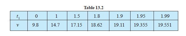
From Table 13.2, we observe that the average velocity is gradually increasing.

Hoping that nothing really dramatic happens between `1.99` seconds and `2` seconds, we conclude that the average velocity at `t = 2` seconds is just above `19.551m//s.`

Compute the average velocities for various time intervals starting at `t = 2` seconds. As before the average velocity `v` between `t = 2` seconds and `t = t_2` seconds is

`= ( "Distance travelled between 2 seconds and seconds " ) /["Time interval " (t_2 –2 )]`

`= ( "Distance travelled in seconds - Distance travelled in 2 seconds " ) / (t_2 –2 )`

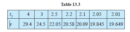
The following Table `13.3` gives the average velocity `v` in metres per second between `t = 2` seconds and `t_2` seconds.



In the first set of computations, what we have done is to find average velocities in increasing time intervals ending at `t = 2` and then hope that nothing dramatic happens just before `t = 2.`

In the second set of computations, we have found the average velocities decreasing in time intervals ending at `t = 2` and then hope that nothing dramatic happens just after `t = 2`.

Purely on the physical grounds, both these sequences of average velocities must approach a common limit.

We can safely conclude that the velocity of the body at `t = 2` is between `19.551m//s` and `19.649 m//s.`

Technically, we say that the instantaneous velocity at `t = 2` is between `19.551 m//s` and `19.649 m//s`.

`color{green} "As is well-known, velocity is the rate of change of distance."`

From the given data of distance covered at various time instants we have estimated the rate of change of the distance at a given instant of time. We say that the derivative of the distance function `s = 4.9t^2` at `t = 2` is between `19.551` and `19.649.`



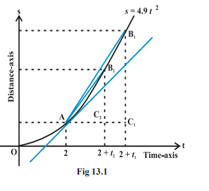
In the limit as the sequence of time intervals h1, h2 approaches
zero, the sequence of average velocities approaches the same limit as does the sequence of ratios

`(C_1B_1)/(AC_1), (C_2B_2)/(AC_2),(C_3B_3)/(AC_3)`

Consider the function `f(x) = x^2.`. Observe that as `x` takes values very close to `0,` the value of `f(x)` also moves towards `0`

`lim_(x->0)f(x) = 0`

(to be read as limit of `f (x)` as `x` tends to zero equals zero).The limit of `f (x)` as `x` tends to zero is to be thought of as the value `f (x)` should assume at `x = 0.`

In general as `x → a, f (x) → l,` then `l` is called limit of the function `f (x)` which is symbolically written as `lim_(x->a)f(x) = l`.

Suppose `y=f(x)`

This relationship can be visualised by drawing a graph of function `y=f(x)` as shown in Fig. (a).

Consider the point `P(x,y)` and point `Q(x+Deltax, y+Deltay)` on the curve `y=f(x)`.
Slope of line joining PQ : `tan theta=(Deltay)/(Deltax)=((y+Deltay)-y)/(Deltax)`

Suppose now that the point Q moves along the curve towards P. In this process, `Deltay->0, Deltax->0`; though their ratio `(Deltay)/(Deltax)` will not necessarily vanish. This line becomes a tangent to the curve at point P as shown in Fig. (b).

This means that `tan theta` approaches the slope of the tangent at P, denoted by m:
`m=lim_(Deltax->0) (Deltay)/(Deltax) = lim_(Deltax->0) ((y+Deltay)-y)/(Deltax)`

• The limit of the ratio `Δy/Δx` as `Δx` approaches zero is called the derivative of y with respect to `x` and is written as `dy/dx.`

• It represents the slope of the tangent line to the curve `y = f (x)` at the point `(x, y).`

Since `y = f (x)` and `y + Δy = f (x + Δx),` we can write :

`(dy)/(dx)=(df(x))/(dx)=lim_(Deltax->0) (Deltay)/(Deltax)=lim_(Deltax->0)[(f(x+Deltax)-f(x))/(Deltax)]`

Suppose a variable force `f (x)` acts on a particle in its motion along `x -` axis from `x = a` to `x = b.` The problem is to determine the work done `(W)` by the force on the particle during the motion.

• If the force were constant, work would be simply the area `F (b-a)` as shown in Fig. (i).

• If force is varying, To calculate the area under this curve [Fig. (ii)], divide the interval on x-axis from a to b into a large number (N) of small intervals: `x_0(=a)` to `x_1`, `x_1` to `x_2`, `x_2` to `x_3`, ............`x_(N-1)` to `x_N(=b)`.

The area under the curve is thus divided into N strips. Each strip is approximately a rectangle, since the variation of F(x) over a strip is negligible.

The area of `i^(th)` strip is approximately `DeltaA_i=F(x_i) (x_i -x_(i-1))=F(x_i) Deltax`
The total area under the curve `A=sum_(i=1)^N (DeltaA_i) = sum_(i=1)^N F(x_i) Deltax`

The limit of this sum as `N->oo` is known as the integral of F(x) over x from a to b. It is given a special symbol as shown below:
`A=int_a^b F(x) dx`

• A most significant mathematical fact is that integration is, in a sense, an inverse of differentiation.

Suppose we have a function `g (x)` whose derivative is `f (x)`, i.e. `f(x)=(dg(x))/(dx)`
The function `g (x)` is known as the indefinite integral of f (x) and is denoted as: `g(x)=intf(x)dx`

• An integral with lower and upper limits is known as a definite integral. It is a number.
• Indefinite integral has no limits; it is a function.

• A fundamental theorem of mathematics states that `int_a^b f(x)dx=g(x)|_a^b =g(b)-g(a)`

`d/(dx) (sinx ) = cos x \ \ \ \ : \ \ \ \ d/(dx) (cos x ) = - sin x`

`d/(dx) (tan x) = sec ^2x \ \ \ \ : \ \ \ \ d/(dx) (cot x ) = - cosec^2x`

`d/(dx) (sec x ) = tan x sec x \ \ \ \ : \ \ \ \ d/(dx) (cosec^2x ) = - cot x cosec x`

`d/ (du) ( e^u) = e^u`

`color(blue)(★ul"Multiplication by constant")`

`(d (a u ) )/(dx) = a (du ) /(dx) \ \ \ \ : \ \ \ \ (du )/(dt) = (du)/(dx) * (dx)/(dt)`

`color(blue)(★ul"Power Rule ")`

`d/(dx) (u)^n = n u ^(n -1) (du)/ (dx) \ \ \ \ : d/ (du ) ( ln u ) = 1/u`

`d/(dx) ( x^n) = nx^(n-1)`

`color{green}"Example :"`` f(x) = 8 x^5 + 4x^4 + 6^3 + x +7`

`d/(dx)f(x) =f'(x) = 8 (5)x^(5-1) + 4 (4) x ^(4-1) + 6(3)x^(3-1) + x^(1-1)`

`f'(x) = 40 x^4 + 16x^3 + 18x^2 +1`

`color(blue)(★ul"Product Rule")`

`(d(uv))/(dx) = u (dv)/(dx) + v (du)/(dx) `

`color{green}"Example :"` `f(x) = x^3 cosx`

`d/(dx)f(x) =f'(x) = x^3 d/(dx) (cos x) +(cos x) d/(dx) (x^3 ) `

`f'(x) = x^3 ( -sinx ) + 3 x^2 cos x`

`color(blue)(★ul"Quotient Rule ")`

`(d(u//v))/(dx) = [v (du)/(dx) - u (dv)/(dx)]/v^2`

`color{green}"Example 1 :"` `f(x) = x /(x +1)`

`d/(dx)f(x) = f'(x) = (( x+1) (d(x))/(dx) - (x) (d)/(dx)(x+1) )/(x+1 )^2 = 1/ (x +1)^2`

`color{green}"Example 1 :" ``f(x) = x^2/(sinx)`

`d/(dx)f(x) = f'(x) = ( sin x(d)/(dx) (x^2) - (x^2)(d)/(dx)(sinx))/(sinx)^2 = (2x sin x - x^2cos x)/(sin^2x)`

`(du)/(dv) = (du//dx)/(dv//dx)`

`color{blue}{ int x^n dx = (x^(n +1)) / (n +1) }\ \ \ \ \ \ (n != -1 )`

`color{green}"Example :"` `f(x) = x^4 + 3x^2 + x +1`

`int f(x) dx = 8 int x^4 dx + 3 int x^2 dx + int x dx + int 1 dx`

`int f(x) dx= (8x^5)/5 + (3x^3)/3 + x^2/2 +x`

`int f(x) dx= 8/5x^5 +x^3 + 1/2x^2 +x`

`color{blue}{ int (1/x) dx = ln x} \ \ \ \ \ \ ( x > 0 )`

`color{blue}{ int sin x dx = - cos x \ \ \ \ \ \ int cos x dx = sin x}`

`color{blue}{ int e^x dx = e^x}`